An Algorithm to Generate Color Palettes
So you’re looking for a beautiful color palette for this website you’re working on? Maybe you recently equipped your house with RGB lighting or you’re about to paint your living room walls with some fresh colors? You just got this shiny new LED keyboard and want to make full use of its features? In my case it was a combination of all of these.
Whatever your situation might be, if you are just a tiny bit like me, you feel like you’re constantly tweaking your color schemes. You want a decent color palette, something a bit more charming and appealing than just plain red, green and blue. (Yes, yes, I hear you. I’ll have to change my blog’s sidebar color)
math.Rand
Being a programmer, I quickly wrote a few lines of code to generate random color palettes. Already aware that this approach might not yield the best results, I prepared for a couple of minutes of frantic “reload” key smashing. Surely I’d just need a bit of luck and patience and would be rewarded with a beautiful color theme that I would instantly fall in love with.
Boy was I wrong. Generating color palettes from random color values sucks: every now and then it would produce a lovely color, just to pair it with the ugliest, muddiest hues of brown or yellow. You would always end up with a selection of colors way too dark or way too bright, one that offered too little contrast or a palette where the colors looked too similar to another. There had to be a better way.
Color Spaces
Let’s start with the theory. There are a few commonly used color spaces to classify colors:
sRGB
RGB stands for Red Green Blue. This is how your computer screen works: it
emits a colored light for each of the three color channels, which blend together
as you perceive them. Each channel’s value ranges from 0 to 255. R:0, G:0, B:0
(or #000000 in hex) is black, R:255, G:255, B:255 (or #ffffff) is white.
CIE Lab
The CIE Lab color space has
a wider range than sRGB and includes all humanly perceivable colors. It is
designed to be perceptually uniform. In other words, the distance between colors
in this space is a perceptive distance: if two colors' values are close to each
other, they will also look similar to you. Two distant colors, on the other
hand, will also be perceived as distinct colors. In CIE Lab there’s more room
for saturated colors compared to darker or lighter ones. To your eyes, a very
dark green is almost indistinguishable from a black, after all. This color space
is also three-dimensional: L represents the lightness (between 0.0 and 1.0),
whereas a & b (roughly between -1.0 and 1.0) are the color channels.
HCL
If RGB is how screens produce colors and CIE Lab is how we perceive colors,
HCL is the color space that
most closely resembles how we think about colors. Like the other two color
spaces it’s three-dimensional, and uses the values H for Hue (between 0 and
360 degrees), C for Chroma and L for Luminance (both between 0.0 and 1.0).
If there’s just one thing you’re going to remember from this blog post, let it be that you should use the CIE Lab color space for computations and HCL when presenting color palettes to the user. You can eventually convert values from those color spaces to RGB, should you really need them in that format.
Partitioning a Color Space
As I want a set of unique, distinct colors, let’s first eliminate those that
we perceive as too similar. The color space we want to operate in is
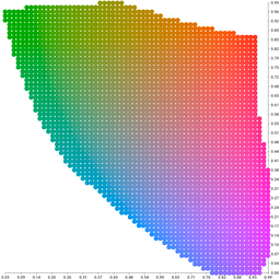
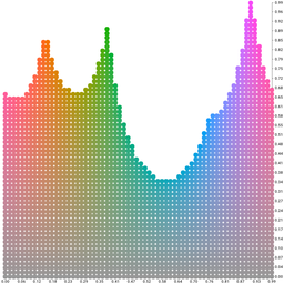
three-dimensional, and the k-means clustering
algorithm is a fantastic way to divide such low-dimensional data sets. It tries
to partition the provided data points (in this case our color space) into k
distinct areas. The palette is then made up from the clusters' center points in
these areas. The visualization to the right is a two-dimensional plotter output
of the algorithm at work in the three-dimensional CIE Lab color space.
Let’s Write Some Code
With the Go implementation of the k-means algorithm, this problem can be solved in just a few lines of code. First, we want to prepare a data set with the color values in the CIE Lab space:
|
|
As you can see, we can already tweak a couple of parameters and apply certain constraints to the colors we want to be generated. In this example we exclude colors that are either too dark (lightness <0.2) or too bright (lightness >0.8).
Let’s partition the color space we just created:
|
|
The Partition function will return a slice of eight clusters. Each cluster has
a Center point which represents a distinct color in the given color space. You
can easily translate its coordinates to an RGB hex value:
|
|
Remember that the CIE Lab space has a wider color range than RGB, and therefore
certain Lab values have no representation in the RGB space. Clamped converts
those values to the closest matching color in the RGB spectrum.
Complete Example
|
|
A set of eight (not so) random colors generated by the code snippet above:
Define Your Own Color Space
We want a little more control over the colors we generate, though. Luckily it’s easy to control the data set we compute on and bend the color space to our needs. Let’s generate some milky Pastel colors:
|
|
Yet another color space: HSV, which stands for Hue, Saturation and Value (brightness). You can look up the details on Wikipedia, but what’s important here is that Pastel colors in this space typically have high values for brightness, but low saturation.
The Pastels it generated:
Similarly, you can filter colors by their chroma and lightness to extract a set of “warm” colors:
|
|
Generates:
The gamut Package
I’m currently working on a library called gamut, where I’ll combine all the bits and pieces presented here into one convenient package that lets you generate and manage color palettes & themes in Go. You can already play with it, but it’s still work in progress. Stay tuned. More about gamut in the next blog post.